Documentation
Deep-LASI comes with an interactive graphical user interface (GUI) to perform processing and analysis tasks during the data evaluation. This page serves for documenting its functionalities. Deep-LASI comes with six integrated GUI sub-windows for analyzing the data and one menubar for handling the data reading, the settings of the program, and simulating single-molecule data. The analysis-GUIs are dedicated to (1) opening files and molecule identification, (2) mapping and trace extraction, (3) trace categorization, selection, trace correction/analysis, (4) SNR analysis of traces, (5) the summary of the results including FRET, states, correction factors and TDP plots, and (6) the classical HMM analysis via different software packages.
To start learning how to use Deep-LASI, we recommend, first, reading through the How to get started and Example Galleries sections. A step-wise description of how to analyze different single-molecule data with Deep-LASI is given for selected showcases in the Example Galleries in detail.
Overview
Data requirements
Data handling
Deep-LASI incorporates single molecule data at different levels. First, it reads movies from emCCD or sCMOS cameras, as usually acquired using a wide-field total internal reflection fluorescence (TIRF) microscope. Consecutively, it extracts the intensity information of single and co-localizing molecules depending on the excitation scheme and assay and saves the extracted traces afterward. For already recorded intensity time traces from confocal microscopy and localization microscopy, Deep-LASI imports the trajectories as formerly saved without additional correction. Fig. 2 summarizes the data handling.

Fig. 2 Workflow summarizing the generic data formats used by Deep-LASI, as well as supported data formats for trace import.
Supported Data Formats
Deep-LASI was developed to handle movie files containing single-molecule data. Nevertheless, it can also import recorded data from other sources (see below). We are happy to support further standard image formats to make Deep-LASI compatible with other systems and software packages. For more specialized / home-built setups and data formats, we recommend first reading the custom-file section before getting in touch with us in the Forum and/or via …
TIFF, Tagged Image File Format (.tif)
Deep-LASI accepts movie files in the Tagged Image File Format (.tif). These files can contain stacks of wide-field/TIRF images with one or multiple detection channels for different laser excitation schemes. Choose this file format if you want to load raw data from, e.g., emCCD cameras.
PicoQuant universal file format (.ptu)
Deep-LASI can handle confocal data obtained by scanning laser microscopy in ‘Pick-n-destroy’ mode. Single time traces saved in the PicoQuant universal file format (.ptu) can be read consecutively. So far only single-channel read-in is supported and tested on .PTU files recorded using HydraHarp Software V3.0.
Hierarchical Data Format 5 (.hdf5)
To analyze data files from localization microscopy extracted and generated with Picasso, we extended Deep-LASI also to read in the binary file format Photon-HDF5 (.hdf5) as described on http://photon-hdf5.github.io. For every localization event the raw photon stream is loaded, while missing localizations set the default to 0 intensity.
Custom file formats
The vast number of different commercial and custom-built microscope setups makes it fairly impossible to host all data and file formats that could be analyzed in Deep-LASI. We, therefore, designed a spot in the file type selection for a custom read-in routine. These routines are saved in the import folder and must be a MATLAB file (.m) with a specific structure which can be found in all other import functions.
Saved File Formats
For data import and storage, Deep-LASI saves and handles three further file types:
Format |
Data Types |
|---|---|
*.mat |
File containing the extracted or imported traces |
*.tdat |
File containing the mapping information and saved data sets |
*.npz |
File containing simulated traces |
Files ending with .mat contain extracted or already imported traces. Mat-Files are the standard format by Deep-LASI using the MATLAB Data format. How to access and/or read, this data externally is described in more detail in Data structure.
Files ending with *.tdat are generated after mapping different detection channels. They contain information about how camera images between different channels refer to each other, i.e., about potential translational and rotational offsets, as well as differences in magnification. Mapping files are generated before trace extraction, usually via a separate movie showing a calibration pattern or multi-labeled particles, and used for matching single-molecule co-localizations between different channels.
Files ending with *.npz refer to simulated single-molecule traces as described in the Simulations page. They are read in directly for trace analysis.
Data structure
Most data in Deep-LASI is stored as global variables in the background to allow easy access. They are saved in the transportable structure T, which can be extracted at any point of the analysis to the workspace by typing >> global T in the command line of MATLAB. The most important variables are:
Variable |
Content and format |
|---|---|
T.Channel |
Container for all the information for each camera |
T.Channel.Traces |
All intensity and FRET traces sorted according to the excitation cycle |
T.ALEXsequence |
Excitation color for each frame |
T.FrameTime |
Exposure time including frame transfer |
T.HMM |
Container for all parameters and results obtained from Hidden Markov models |
T.NeuralNetwork |
Container for all loaded neural networks and prediction results |
Data Import from OT and TRACY
This function is for internal use within the hosting group only. Deep-LASI allows for importing FRET data obtained from Multi-Color Orbital Tracking measurements using the setup specific data format.
TRACY was the former software for the evaluation of 1c and 2c FRET traces. Deep-LASI allows for importing the formerly exported and evaluated traces, as well as exporting new data sets into the old format.
Processing Single-Molecule Data
Starting Deep-LASI
To evaluate your experimental data with Deep-LASI, please open the program from the MATLAB command window by typing in >> DeepLASI. It will open the core program responsible for data import, trace extraction, as well as manual selection and sorting. After a couple of seconds, the Start-GUI of the program will open as shown in Fig. 3.

Fig. 3 The Main-GUI of Deep-LASI has six sub-windows for data processing and analysis.
Deep-LASI shows one empty Main-GUI together with six integrated sub-windows for analyzing the data and one menubar for handling the data reading, the settings of the program, the simulation of single-molecule data, and training (new) neural networks.
Menu Bar
Basic functionalities of Deep-LASI, such as data handling, program settings, or the training of new neural networks for data analysis, are controlled via the Menu Bar. It has the following five drop-down menus
File |
Functions for loading, mapping, processing, saving, importing and exporting data |
Settings |
Access to Camera Settings |
View |
Appearance of the GUI, Graphs and Data representation |
Tools |
Programs for accessing/simulating single-molecule data, and training Neural Networks |
Help |
Direct link to the Documentation in case of problems |
Reset |
Restart of Deep-LASI and clearance of all variable of the program |
Dropdown Menu File.
The dropdown menu File (Fig. 4) controls all steps, starting from loading the experimental data, over mapping and background correction, to trace extraction and saving of traces. Moreover, it facilitates data import and export in different formats, as described in the Data requirements section. The dropdown menu hosts seven sub-routines:
The sub-routines in Mapping are used to match the corresponding image pixels between up to four different cameras. They allow the user to generate, save and reload maps containing the transformation matrices between the channels. A description of how to map the detection channels is given below in the Mapping section.
Load Image Data facilitates the read-in of data files per detection channels. The data needs to be read in consecutively, starting with Channel 1 being the most ‘blue’-shifted detection channel and Channel 4 being the most ‘red’-shifted detection channel. Data loading is possible for a single file per channel, but also for multiple files at once. Please make sure: (1) that the numbers of loaded files per detection channel match and (2) that the files have consecutive numbering so that corresponding movies are loaded.
Using the Load Traces/State routine, previously extracted and potentially already evaluated traces can be reloaded into Deep-LASI.
The Add Traces/State routine allows the addition of further extracted traces to already loaded traces. This function is especially useful for merging trajectories from various measurements. Please note that only traces with identical experimental settings (e.g., number of frames, exposure time, or laser excitation) can be merged.
Save Traces/State to save desired changes on traces, for example, if you have already carried out all analysis steps.
The Import function allows loading data sets from other single-molecule measurements (as described in the Data requirements section above). The imported traces are only loaded and not further modified by Deep-LASI.
Export allows for transferring extracted traces to a former analysis software used by the hosting group and to save and export traces and enables the saving of single trajectories in graphic formats.
Quit terminates the program.

Fig. 4 Deep-LASI file menu
Dropdown Menu Settings.
The dropdown menu Settings (Fig. 5) opens a sub-window for entering the camera hardware settings chosen in the experimental setup. The routine asks for the EM Gain factor, the camera baseline in dark counts, and the number of photons per camera count for each camera. With this, Deep-LASI can convert/display the determined intensity instead of arbitrary units in Counts per second, i.e., in Hertz.

Fig. 5 Deep-LASI settings menu
Dropdown Menu View.
The third dropdown menu View controls the appearance and settings of the graphical interfaces on the different GUI sub-windows of Deep-LASI.
The sub-tab Colormap changes the color palette in 3D plots, e.g., on the Trace GUI surface (which shows small zoomed-in areas of 24x24 pixels) or the Extraction GUI surface (which shows the average projection of localized molecules). In both cases, localized molecules are highlighted. The default colormap is jet, which can be exchanged by other standard color maps from MATLAB.
The Plot Units sub-tab controls the y-axis of the intensity and FRET panels for individual single-molecule trajectories. Checking/unchecking the different sub-tabs immediately updates the graphical interface and the way how a single-molecule trace is displayed. The sub-tab Plot Units provides the following four different settings for displaying intensities and FRET trajectories:
Photons (Cam. calibrated) |
Intensity is shown as the absolute number of photons |
Mean across Particle Mask |
Intensity is shown as mean intensity within the detection mask |
Raw Trace (no BG subtr.) |
Intensity without background correction |
Corrected FRET |
Display of accurate FRET instead of apparent FRET |
The first sub-tab, Photons (Cam.calibrated), converts the intensity axis into the absolute number of photons being detected by the individual cameras during a particular excitation cycle. It updates the intensity axis of extracted single-molecule traces on the Traces GUI window.
The second sub-tab, Mean Across Particle Mask, shows the mean emission intensity of the particle within the detection mask after trace extraction on the y-axis of the single-molecule traces on the Traces GUI window.
The penultimate sub-tab, Raw Trace (no BG subtr.), activates the display of uncorrected, raw intensity traces, i.e., without background subtraction.
If the last option, Corrected FRET, is selected, Deep-LASI shows Accurate FRET efficiencies for each single-molecule trajectory in case the FRET correction factors have already been determined. Otherwise, the displayed FRET values between Accurate and Apparent FRET are identical.
Dropdown Menu Tools.
The fourth dropdown menu Tools opens the sub-panels for simulating single-molecule traces and training neural networks. A detailed description of its functionalities, workflow, and usage is given in the Simulations Chapter.
Dropdown Menu Help.
In the case of problems or errors, help can be found in the dropdown menu Help, which provides a direct link opening this Online documentation of Deep-LASI.
Dropdown Menu Reset.
When finishing the analysis of one data set, a change to a new data set can create errors, in particular, if they differ with respect to laser alternation, imaging modalities, or the number of emitters. In this case, please reload the program via the Reset button. DeepLASI will reset all temporal variables in the background, refresh the graphical interface and restart the program.
Main-GUI
Data analysis with Deep-LASI involves consecutive working steps (Fig. 6), which are accommodated in six different sub-GUIs, as shown in Fig. 3. The Starting-GUI incorporates single molecule data at different levels. First of all, it reads movies from emCCD or sCMOS cameras, as usually acquired using a wide-field total internal reflection fluorescence (TIRF) microscope, and maps corresponding pixels between cameras onto each other (see the section on Mapping). Next, it extracts the intensity information of single and co-localizing molecules depending on the excitation scheme and assay and saves the extracted traces afterward, as described in more detail in the section Trace extraction. For already recorded intensity time traces from confocal microscopy and localization microscopy, Deep-LASI imports the trajectories as formerly saved without additional correction. Equally, already extracted traces can be loaded into Deep-LASI for further data analysis.

Fig. 6 Workflow summarizing the generic data formats used by Deep-LASI, as well as supported data formats for trace import.
The main data handling is carried out on the Traces GUI (Fig. 6). Here, you can choose between manual or automated data analysis. Conventional data analysis includes sorting, categorization, and trace preparation (as described in the section Traces GUI) before handing over the preselected traces for Hidden-Markov modeling on the HMM GUI followed by dwell time analysis and TDPs. The sub-window Histograms allows for summarizing the analyzed data via histograms with respect to, e.g., frame-, molecule-, and state-wise histograms, or the global FRET correction factors (Fig. 6). The sub-window Statistics on selected molecule groups with respect to, e.g., average brightness, background, SNR, etc.
The automated data analysis is carried out on the Traces GUI, which includes an automated selection, sorting, and categorization process prior to an automated kinetics analysis based on deep learning. The data is afterward automatically summarized by state-of-the-art dwell-time analysis and TDPs.
Mapping
Before loading data into Deep-LASI, one needs to consider the experimental requirements. In the case that single-color data has been acquired, the data can be directly loaded into the software, and single-channel traces can be extracted, as described in Trace extraction. In the case that more than one detection channel has been employed, we need to know where the emission of labeled molecules is detected on the different field-of-views (FOV) of the cameras, i.e., which pixels on one channel correspond to pixels on the other (Fig. 7).

Fig. 7 Mapping between multiple detection channels copes with differences between the FOV due to translation, rotation, and magnification.
For mapping the different channels onto each other, please go to the dropdown menu File and choose
> File > Mapping > Create New Map and load the reference data stepwise into Deep-LASI by clicking on > 1st channel. The first channel refers to the FOV with the most blue-shifted emission, e.g., blue emission in a BGR ALEX excitation scheme. In the case that you use a split camera for two detection channels, you need to load the movie twice for the two corresponding channels separately and select the corresponding halves of the FOV in a consecutive step.
Next, the program will ask you to choose a file which could be an image or a series of images as a video file. This reference data should contain structures or emitters with multiple co-localization on the various cameras. This could be, for example, a cover slide with multi-colored beads or DNA origami structures with multiple labels. The emitters should be dense (but well separated) and widely spread over the entire FOV, such that aberrations in all areas of the FOV can be correctly translated between the different detection channels.

Fig. 8 Uploading first mapping image
After choosing the calibration file, Deep-LASI opens a window (Fig. 8), which allows you to determine the correct position of the detection channel. You can use the Channel Layout to select the correct half of the camera or the full width of the camera. Rotation and Flip allow you to take into account if your camera image is flipped or rotated compared to your reference channel. After the selection, please confirm OK to open the image on the mapping tab, as shown in Fig. 9.

Fig. 9 Selection of recognized emitters in the first detection channel by Deep-LASI
After loading, use the threshold bar below the loaded image to make sure that enough points are detected (indicated by the white circle) by Deep-LASI. Next, continue opening the following images from other detectors by selecting the > 2nd channel, etc., via the same procedure as shown in Fig. 8 and Fig. 9.
Once you have loaded all mapping images to assign the detection windows, please select afterward which channel you prefer to be the reference channel, as shown in Fig. 10. In most cases, the first channel is taken as the reference unless you have a special mapping plan. In the case that you experience a lot of photo-bleaching, mapping onto the channels with the most emitters might be advisable.
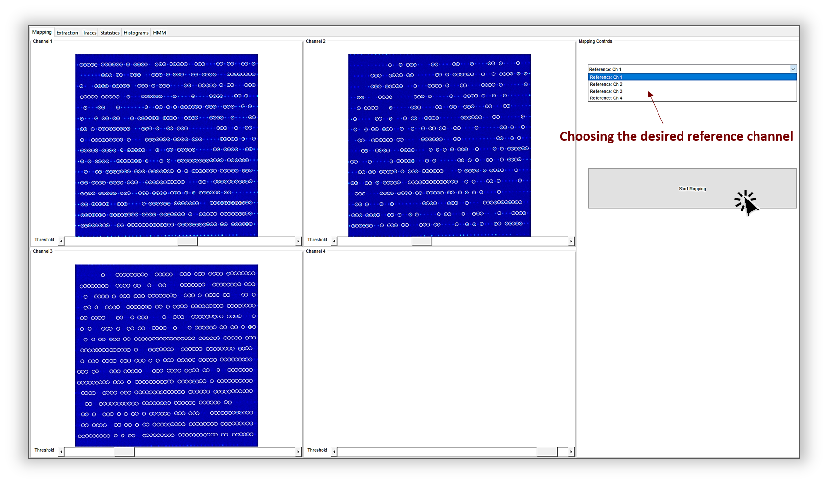
Fig. 10 Performing the mapping step
Once you confirm your selection by clicking on Start Mapping, Deep-LASI aligns the different channels compared to the chosen reference channel and warps the presented images. Deep-LASI describes this mapping process by an affine transformation matrix, taking translation, rotation, and scaling into account.
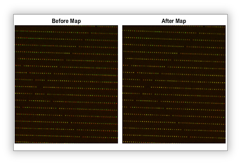
Fig. 11 Mapping result showing the channels overlay before and after mapping
After a successful mapping process, the Extraction-GUI opens automatically. The mapping process itself is fast and visualizes the mapping results as a comparison of image overlays before and after the mapping procedure (Fig. 11). To save the transformation matrix, i.e., the mapping result for any trace extraction later on, finally save the generated map (stored in the memory of Deep-LASI at this point) by clicking on > File > Mapping > Save Map. It is recommended to check the quality of mapping. In some cases, you might have to rerun the mapping process by choosing (1) a different reference channel (e.g., if too many localizations in the different FOVs obscure the mapping process) or (2) a new data set of images (e.g., if too little localizations impede a representative mapping of aberrant images).
Trace extraction
While single-color data can be directly loaded into Deep-LASI, multi-color assays require a mapping procedure first. Once this map is available and saved, you can start extracting experimental data anytime. As shown in Fig. 12, Deep-LASI will match the fluorescence signature from your single fluorophores during different excitation cycles and detection channels (once you have specified the single-molecule assay) and allows you to select which labeled molecules you actually want to evaluate. For this, you first need to step-wise read-in the experimental data, as described in the Loading section. Next, Deep-LASI will generate a projection for each channel, i.e., the corresponding .tif-file, showing the maximum intensity per pixel in the FOV. Deep-LASI will localize single emitters in each of the selected channels and superimpose the three maps afterward, showing the localized molecules in the individual channels. In the last step of the extraction process, Deep-LASI allows you to select whether you want to export all traces (i.e., the trajectories of single-, double- or triple-labeled molecules), traces of only co-localizing molecules (i.e., molecules having the maximum number of traces) or molecules that have a specific label in a reference channel. After a successful extraction process, you are directly forwarded to the third sub-GUI Traces, where you need to save the extracted traces first before continuing with any data analysis.

Fig. 12 Trace extraction of molecules with one, two, or three labels and selection of whether trajectories for all molecules, co-localizing molecules only, or molecules that show emission in a specific channel shall be generated.
Extraction modes
To start the extraction process, reload the earlier derived map via > File > Mapping > Open Map. Once the map is successfully loaded, you are directly forwarded to the sub-GUI Extraction showing a detection mask created like the one shown on the top right part of Fig. 13. Alternatively, you were directly forwarded after the Mapping process (please don’t forget to save the generated map in this case before proceeding with the extraction).

Fig. 13 The mask created after mapping with adjustment options
Before data loading and trace extraction, you first need to consider which kind of experiment has been carried out. Deep-LASI supports the following types of measurement modes:
multi-color measurements with alternating laser excitation
multi-color measurements with constant laser excitation for a fixed number of frames
ALEX excitation
In the case of ALEX excitation, load the data files after mapping the channels, as described in detail in the Example Galleries section. Select one .tif-file or multiple files via > File > Load Image Data > Channel 1 and let Deep-LASI read the data.
Next, specify the measurement parameters of the ALEX experiment (Fig. 14), such as the inter-frame time and alternation cycle. The inter-frame time should include the exposure time and frame transfer time, e.g., when measuring a frame transfer time of 2.2 ms and exposure time of 50 ms by the emCCD camera, the total inter-frame time amounts to 52.2 ms.

Fig. 14 The window for specifying measurement parameters and excitation scheme
Please specify the sequence of the laser excitation using the letters B (blue), G (green/yellow), R (red), and I (infrared) for the four excitation channels. Different excitation schemes of up to three lasers can be entered here, such as RGB, RG, GB, etc. In the case of ALEX excitation, all channels are shown in the preview according to the created map, and the selected channel for data read-in is highlighted by a rectangle. Move the slider to choose the start frames of your entered excitation scheme and load it into the corresponding detection channel. This slider serves for movies where the starting point of data acquisition varies with laser excitation. For a varying acquisition, every single tif.-file needs to be loaded separately to select the correct alternation sequence / starting frame. The slider has 2 positions for a 2c-ALEX experiment. It automatically shows 3 positions in the case of a specified 3c-ALEX experiment.
Next, please choose which frames you want to load on the program using the Load frame range box. Depending on the experiment, you can choose the range of desired frames for detecting the particles and extracting their intensity traces. Deep-LASI takes all the frames by default. You can further limit the particle detection to a certain frame range, e.g., for a colocalization assay in which you used one excitation wavelength for the first 100 frames and continued with a second excitation wavelength for the rest of the measurement. As the last step here, click on the corresponding channel color to confirm the detection channel. Deep-LASI will open the first data file from the files being selected, as shown in Fig. 15, and display the cumulative sum of the movie for particle detection.

Fig. 15 Particle detection for the first channel data
The sliders below the image allow for adjusting the brightness/contrast settings, the detection threshold to register particles, and to change between detection channels during the later extraction steps. Set the slides such that you maximize the number of detected molecules. Localized particles are marked by triangles superimposed on the image, and their localization number is shown in the black box aside from the image on the top right position(Fig. 15).
In the next steps, please repeat loading the recorded data of the other detection channels by selecting the corresponding .tif-files or set of files via > File > Load Image Data > Channel 2, etc. Each time you load image files, the pop-up window will ask you about the detection channel color to extract the data in the correct order.
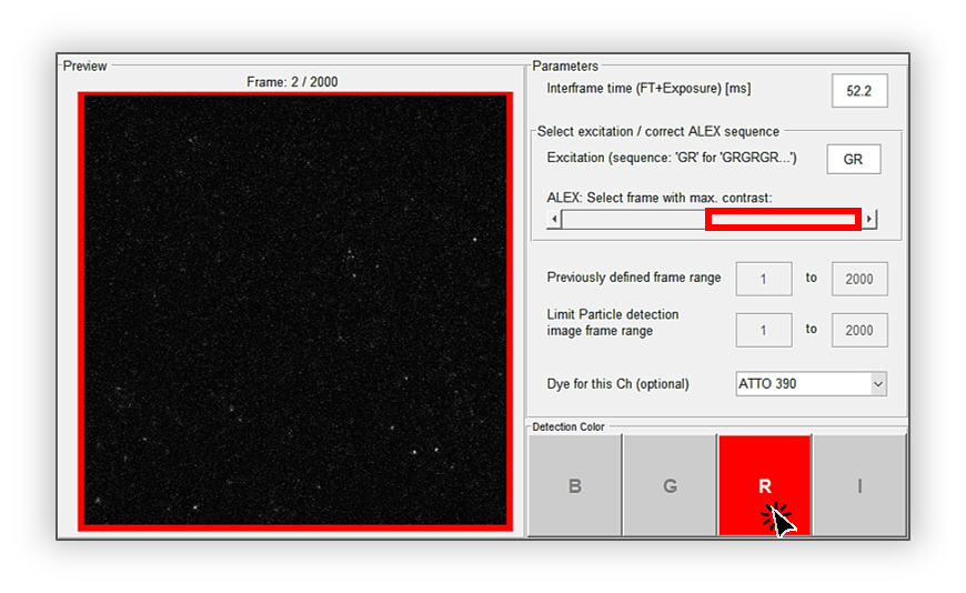
Fig. 16 Updating measurement parameters for the next channel
As shown in Fig. 16, put the slider on the second half of the slider position to indicate the second channel (the same procedure works for the third channel by putting the slider in the right position). The reasoning behind this step is again to provide the freedom to select the correct excitation. Afterward, click on the red button labeled with ‘R’ (as specified in the alternation cycle box to confirm the acceptor channel. After a short time the average imaging of the specified loaded frames of the second channel overlays on the image from the first one.

Fig. 17 Detection of particles and their co-localization
Once all desired channels are loaded and all detection channels have been identified, you can specify how you want to extract traces and which frame range. In the Mask setting panel, you can choose how the background and intensity of the single emitters shall be extracted (Fig. 18). In the Mask drop-down menu you can choose between Manual and Autocorr. PSF. Depending on the chosen Mask the following three parameters PSF, BG inner and BG outer have different meanings. For the Manual Mask, the editable values specify the diameter of the PSF, the BG inner ring and BG outer ring as a ratio of the total cut out radius (19 pixels). The pixels between the inner and outer BG ring will be used for the background calculation. Choosing the autocorr. PSF will use the Fourier transform of the loaded image to determine the particle shape. Here the PSF, BG inner and BG outer values are used as a threshold in fourier space to determine the corresponding radii.
Next, specify which methods for particle detection shall be employed:
Wavelet detection (see for example Messer et al. or Ganjalizadeh et al.)
Intensity Thresholding (spatial bandpass denoising and extraction of centroids based on intensity)
Regional Maxima (intensity thresholding with additional radial center refinement using the in-built imregionalmax function)

Fig. 18 Determining the mask settings and trace extraction method
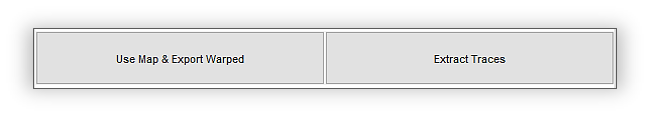
Fig. 19 Provided modes for extracting traces
All particle detection methods undergo a center offset refinement using gaussian filtering with a 3 pixel tolerance.
Lastly, specify in the Trace selection panel which traces you wish to extract. As indicated by the colors of the triangles (Fig. 17) for each corresponding channel, you can extract either (1) all detected emitters independent of the detection channels (e.g., donor only, acceptor only, and FRET pairs) or (2) only co-localizing molecules as indicated by the white circles (e.g., only FRET species) or (3) extract the intensity in reference to a selected channel, which could be donor only species together with FRET species. The panel Frame selection allows for setting the frame range in which traces shall be extracted. In the case, you wish to export the mapped single-molecule image displayed in the Extraction GUI before you finally extract the traces, press the Use Map & Export Warped button on the left at the bottom of the GUI (Fig. 19). For trace extraction itself, click on the right button Extract Traces. DeepLASI will now automatically extract traces movie-by-movie-wise for the file(s) you selected earlier. This process can last several moments but is fully automatically carried out. Once the extraction process is finished, the traces are saved automatically to the last used directory. You can change all following analysis states via > File > Save Traces / State
Note
In the case that an error occurs at the end of the data extraction, try to save the extracted traces anyway. Errors were reported for certain Windows installations that we are currently investigating to solve the problem.
Constant excitation
In the case of constant laser excitation, we must consider different experimental schemes again. When multiple detection channels have been employed during constant excitation with one laser source, …
Tip
@Simon: Please describe here, what you implemented, and how/what we need to fill in, in order to extract traces with constant laser excitaion with different lasers for fixed frame ranges!
Manual smFRET analysis
Single-molecule data analysis using Deep-LASI is carried out in a fully automatic way. However, for new experimental systems, e.g., when studying a new protein system with unknown folding behavior, it is highly advisable to not go for an automatic analysis directly but to analyze the data manually and inspect the recorded traces by eye.
Hence, the following section gives an overview of how to use Deep-LASI manually to sort, categorize and prepare single-molecule data via the sub-GUI Traces (Fig. 20) for later evaluation, e.g., by Hidden-Markov analysis, etc. Automatic data evaluation is described in a separate section on Automatic smFRET Analysis.

Fig. 20 The sub-GUI Traces of Deep-LASI serves for data processing and pre-analysis and serves as starting point for automatic data analysis.
Loading
Starting point of any data evaluation is the loading process from ‘freshly’ extracted traces or traces that shall be re-evaluated. Please load traces via > File > Load Traces. When you recorded multiple datasets with deviating starting frames during alternating laser excitation, please first extract traces for every single movie and then load the extracted traces file-wise via reading the traces of the first file via > File > Load Traces. and adding traces from the other files afterward via > File > Add Traces.
Traces GUI
After data loading, traces will open/show up on the sub-GUI called Traces as shown in Fig. 21 for example for two- or three-color FRET measurements with alternating laser excitation. The GUI is split into two sections: the left part displays the single-molecule data, and the right part is dedicated to trace classification, preparation, sorting, data correction, and automated data analysis, as described later in this Chapter.
Fig. 21 Exemplary single-molecule traces for a (top) two-color and (bottom) three-color FRET measurement.
Trace representation
Depending on the measurement type and amount of detection channels, up to three sub-panels will open up on the left side of the Traces GUI showing the intensity trajectories of a multi-labeled molecule in the upper panels. Their corresponding intensity projections are shown on the right side next to the trajectories. The panel on the bottom left shows the potential FRET signature for different dye pairs. Additionally, Deep-LASI shows small snippets in the column right next to the intensity traces showing the average movie projection in which multi-labeled molecules were found in the different detection channels including their corresponding area chosen for the background determination.
For a two-color FRET experiment (Fig. 21; top), the upper left panel shows the time trace of both, the emission of the donor and acceptor after direct excitation (DD and AA), as well as the sensitized emission (DA), while the corresponding FRET trace is shown on the lower panel on the left. For a single-color experiment, the upper left panel in Fig. 21 will show only one channel , while the corresponding panel for FRET traces will remain empty. Furthermore, Deep-LASI presents the total intensity given as the sum between the DD and DA channel as an additional dark grey/black trajectory. It should be a straight line after correcting against leakage, direct excitation, and detection sensitivity as described in the section Correction factors determination.
Depending on the selected laser excitation scheme during the extraction process, e.g., by choosing BG instead of GR, Deep-LASI will present dual- or triple-color FRET data in different color schemes but with (of course) identical intensity values. The chosen color schemes are summarized in the table below. The detection channel XY refers to the emission in the channel Y after excitation with color X, i.e., the acceptor emission in the red channel after blue excitation is abbreviated with BR:
Detection Channel |
Color |
|---|---|
BB |
dark blue |
BG |
cyan |
BR |
magenta |
BI |
|
GG |
dark green |
GR |
orange |
GI |
black |
RR |
dark red |
RI |
black |
II |
black |
Tip
@Pooyeh/Simon: Please add missing colors
For a three-color measurement, an additional panel displays the trajectories of the detected emitters after excitation with the third laser. As shown in Fig. 21 on the bottom for 3c FRET with BGR laser alternation, the top panel shows three intensities trajectories for the three detection channels after blue excitation, i.e., the emission of the blue dye after blue excitation (BB) in dark blue, the emission of green dye after the blue excitation (BG) in cyan, and the emission of red dye after blue excitation (BR) in magenta. The lower panel shows the emission after green and red excitation. Similar to the two-color case, the color of the different channels will vary depending on which detection channels have been chosen during data extraction. Deep-LASI chooses the above-mentioned color schemes.
You can choose which intensity trace shall be displayed by checking or unchecking channels in the Plot Layout tab in the right lower corner of the GUI. This holds also true for the FRET efficiency signature (which is displayed in the lower panel) or when selecting different regions in the traces, as described in Trace selection. Deselecting FRET channels can become especially handy in the case of having more than one FRET pair per molecule. The Reset Layout button restores the default trace representation.
Trace analysis
The right part of the Traces GUI serves for data handling.
In the Navigation tab, you can switch between traces via the slider.
It displays the currently shown trajectory and the total number of extracted traces. For the 2c-ALEX example, 6100 traces were retrieved from the loaded data set (Fig. 21; top).
The Classification tab serves for the manual categorization of traces. All traces are ‘by default’ in the Uncategorized group. By clicking on the plus sign, you can add more categories. You can rename the new group according to your analysis procedure and further assign keyboard letters via the dropdown menu. The assignment of letters allows for transferring/assigning single traces to the corresponding category by simply pressing the chosen letter on the keyboard when using the keyboard during the manual sorting procedure. An example of possible sorting categories based on our analysis needs is given in Fig. 22. The Create Boolean Category button creates an additional group to the Navigation Tab according to your selection criteria and adds the corresponding traces, which fulfill the condition to the group. You can also delete an unwanted category by clicking on the trash-can icon. Unchecking the filter box hides traces that are already sorted, for example, when clicking through extracted trajectories. It is especially helpful for the trash category, for example. When you assign a trace to a specific category, it will be automatically removed from the first Uncategorized one and added to at least one other group.
Fig. 22 Navigation and categorization box
Note
You can not assign the letters A, D, or E to your categories. These are the keys for going to the previous trace (A) or the following trace (D). Pressing (E), triggers Deep-LASI to automatically find bleaching steps in traces, assign them to the corresponding bleaching group, and select the analysis region, as laid out in the section about Correction factors determination.
The next frame on the GUI comprises two sub-tabs beside the Plot Layout tab, the Deep Learning and Trace tools tabs. The first one allows for hiding or displaying specific emission channels for selected excitation sources, as well as their corresponding FRET signatures, as described above. The Deep Learning tab serves for carrying out automated trace sorting, classification, and analysis, which will be described in Automatic smFRET Analysis. The Trace Tools tab provides you with options regarding to implement correction factors on a current trace or the whole traces Fig. 23. Apart from correcting traces, by clicking on Reset Trace, you can reset all the corresponding correction factors, meaning that the trace will be left in the uncorrected format. Set Median button, will set all the correction factors as the global median values calculated by Deep-LASI. It is especially helpful in case of traces that yield no correction factors themselves.

Fig. 23 The tab Trace Tools provides options about implementing correction factors.
Using the boxes Plot X-Limit and Plot Y-Limit, one can set a maximum threshold for visualizing the traces. For example, if traces are 100 seconds long on X axis, and you are interested in the first 50 seconds of it, you can type 50 in the Plot X-Limit box, and by pressing enter, the trace will be shown until the X value of 50. The same procedure works for the Y axis.
The FRET Controls tab displays and controls the FRET correction factors for direct excitation, leakage, and detection sensitivity. Its functionality will be described in the section about Correction factors determination.
Trace categorization
The categorization of traces depends on the actual single-molecule experiment. In the following, we describe important steps for the analysis of a dual-color FRET experiment with alternating laser excitation as an example. Experienced users can certainly carry out different steps of the categorization and selection process in parallel, i.e., on a single-trace basis.
To fast categorize a large number of molecules, we advise first sorting out all unwanted molecules. Create two groups, for example, called Trash and Further analysis first. Depending on whether you want to go through the list of traces using a mouse or the keyboard, assign two separate letters on the keyboard to the two groups. Now go through all traces and sort out unwanted and useful traces. You can switch forward to the consecutive trace by typing D and go backward to the former trace, which is not categorized yet, by typing A. Once a trace is added to a group, it will not appear any longer in the Uncategorized group.
We additionally advise ensuring that you only keep the single-molecule events. For this, please inspect the middle column on the GUI showing the detected particle in each channel. Make sure that only one molecule is shown inside the detection mask in each channel while no emitter is detected inside the ‘background mask’. Otherwise, exclude the trajectory since the false background calculation will lead to miscalculated FRET correction factors and hence, FRET efficiencies.
Sort between Static and Dynamic molecules. Create categories for dynamic or static traces and add each trajectory to one of the two groups. By this step, you can select afterward which traces shall be analyzed by HMM, for example.
Select regions of the trajectories (as described in the following paragraph Trace selection), which will be evaluated later by kinetics or histogram analysis. Traces with manually selected regions will be automatically added to the Manual Selection category.
Mark regions of the trajectories (as described in the following paragraph Trace selection) in which fluorophores bleach. Deep-LASI will add the traces automatically to the following groups: G Bleach, R Bleach, GR Alpha, GR Beta, and GR Gamma.
Trace selection
For selecting regions in traces, either for further analysis or correction factor determination, Deep-LASI uses the mouse as the active tool for marking different areas. Deep-LASI has two different types of selectors: firstly, it allows for choosing specific time windows according to the detection channel (Fig. 24; left), which is required to derive trace-wise correction factors, and secondly, it provides one selector mode (Fig. 24; right), which marks the starting and stopping time points, in between which the kinetics and FRET states shall be evaluated.
Fig. 24 Activated selector types to manually mark areas in traces
When clicking with the mouse on the trace, first the mouse turns into an active cursor for a general selection of time windows, in which the FRET states and kinetics will be evaluated (Fig. 24; right), e.g., by HMM later on. Once the general selector is active, detection channel-specific selection is accessible by pressing the key 1, 2, or 3 on the keyboard, depending on how many detection channels are available. By pressing the same key again, the cursor will turn into a general selector again. Clicking into the Traces sub-GUI aside the trajectory will deactivate the selector tool.
To select specific areas in traces, one needs to click into a trace with the left button of the mouse, and drag the mouse to make the selected region shadowed, for example, from the beginning of a trace until a bleaching step. Correction or deselection of marked areas is achieved by clicking with the right button into the trace and deselecting the desired time window. Pressing the empty space key on the keyboard will reset all selections and permit restarting of the selection process all over.
The selection process depends on the bleaching behavior of fluorophores and the trace-inherent SNR and photochemical behavior, etc. Detection channel selection is required to determine trace-depending correction factors automatically. If a correction factor can be calculated for a trace, its value will be shown in the FRET control box in the lower right corner. We advise employing as many recorded traces for either of the analysis purposes (FRET evaluation or background correction factors analysis) to obtain significant statistics later on for determining absolute distances after full data correction. We advise marking the time windows with active fluorophores with channel-specific selectors first. A possible FRET evaluation should be selected lastly, as it is not always possible.
Tip
@Simon is the Selection process correctly described?

Fig. 25 Activated cursors for (A-B) channel-specific selection in the green channel (A), in the red channel (B), and for (C) choosing the time window by start and stop value in which the FRET states and kinetics shall be evaluated.
Fig. 25 provides an example of the three selector types available to evaluate a 2c ALEX trace and the outcome of such an analysis. Using the green selector (Fig. 25; A), the time window was marked in which the green dye was active. The middle panel shows the time window in which the red fluorophore was active (Fig. 25; B). The general selector marks the time window for FRET evaluation. This time window is not extra visualized (Fig. 25; C). The FRET efficiency trace gets the selection until the first bleaching step, and this region will be added to the FRET histogram in the end.
Correction factors determination
In real-world single-molecule FRET experiments, the intensity of the acceptor is biased by various sources. It needs to be corrected for direct excitation \(\alpha_{XY;DL}\) of the acceptor dye Y during donor excitation X and spectral crosstalk \(\beta_{XY;DL}\) from the donor molecule X into the acceptor channel Y. Furthermore, we need to correct for the differences in detection sensitivity \(\gamma_{XY;DL}\) between the two fluorophores. We are aware that the nomenclature by Deep-LASI, at this stage, is not in line yet with the nomenclature recently introduced by a multi-laboratory benchmark study published by Hellekamp et al., Nat. Meth (2018). It will be adopted on the various sub-GUIs of Deep-LASI and throughout the software during the next release rounds. Deep-LASI denotes the correction factors currently as
Deep-LASI |
Hellekamp et al. |
Description |
|---|---|---|
\(\alpha_{XY;DL}\) |
\(\delta_{XY}\) |
Direct excitation of the acceptor fluorophore Y during excitation with X |
\(\beta_{XY;DL}\) |
\(\alpha_{XY}\) |
Spectral crosstalk from the fluorophore X in the detector channel Y |
\(\gamma_{XY;DL}\) |
\(\gamma_{XY}\) |
Compensation for difference in detection sensitivities between Channels X |
We denote the background-corrected intensities as \(I_{XY}\) and the corrected intensity as \(I_{XY;corr}\), where X stands for the excitation source and Y for the detection channel.
Trace-wise and global correction factors
Depending on when individual fluorophores photo-bleach, correction factors can be derived on a trace-to-trace basis. For most of the traces, however, only a subset of correction factors can be obtained for the individual trajectories. In these cases, Deep-LASI derives global correction factors, which are the median value of all trace-wise derived correction factors. The distribution of all three correction factors can be visualized on the Histograms GUI, and is described in the section Histogram Analysis and below, respectively.
Deep-LASI uses bleaching steps in single-intensity trajectories to calculate trace-wise correction factors. These can be derived for traces containing bleaching steps, which were presorted and categorized as B Bleach, G Bleach, R Bleach, or I Bleach, respectively, depending on which fluorophore pairs were investigated. The correction factor for direct excitation of the acceptor during donor excitation can be derived for traces in which the donor bleached first or acceptor-only traces, via
where \(\langle I_{XY}\rangle\) and \(\langle I_{YY}\rangle\) describes the mean acceptor intensity after donor or acceptor excitation, respectively. Following the definition of leakage of the donor fluorescence into the acceptor channel according to
Deep-LASI determines \(\beta_{XY;DL}\) from donor-only traces or at acceptor bleaching steps from the static intensity in the donor channel and acceptor channel after the bleaching. Here, \(\langle I_{XX}\rangle\) refers to the mean donor intensity, and \(\langle I_{XY}\rangle\) to the mean acceptor intensity after acceptor bleaching.
Lastly, the detection correction factor \(\gamma_{XY;DL}\) is derived from traces categorized as XY Gamma, in which the acceptor Y is bleaching before the donor molecule X. Before determining \(\gamma_{XY;DL}\), the acceptor intensity \(I_{XY;corr}\) is first corrected against direct excitation and spectral crosstalk. Afterward, Deep-LASI derives the detection correction factor from the ratio of changes in the donor and acceptor emission before and after the photo-bleaching of the acceptor. The correction factor is calculated via
with \(\langle \Delta I_{XX;corr}\rangle\) and \(\langle \Delta I_{XY;corr}\rangle\) being the intensity difference for the mean donor and acceptor emission after donor excitation before and after the acceptor photo-bleaches.
The correction factors calculated for each trace are shown in the FRET control box in the lower right corner of the GUI (Fig. 26; left). For each correction factor a pair value 1 | value 2 is shown, which present the locally derived correction factors and the global correction factor respectively. If a trace is not suitable for calculating any of the correction factors, or if the derived value is totally off, Deep-LASI permits to set a global correction factor. Clicking on the ‘def.’ box in the FRET control panel opens a sub-window (Fig. 26; right). It provides an overview over the mean and mode value of all derived local correction factors including the number of traces, which underlies the statistics. By clicking on the ‘use mean’ or ‘use mode’ box, you can set the global correction factor for the trace. Otherwise, you can also set the correction factor value, by typing in its value in the FRET control panel.

Fig. 26 (Left) Trace-wise correction factors. (Right) After clicking on ‘def.’ in the FRET control panel, a sub-window opens showing the average global correction factors determined from other traces. By clicking on ‘use mean’ or ‘use mode’ the global correction factor values will be employed instead of the locally derived ones.
As shown in the right panel of Fig. 26, in this data set predominantly correction factors against leakage and detection sensitivity were obtained. This is mostly the case, when only the trajectories of co-localizing molecules have been extracted, as described in the Trace extraction section. To obtain a higher statistics for the correction factor against direct excitation in this case, it is advisable to also extract acceptor-only traces.
Once all correction factors are determined, every trace is corrected using the local, trace-wise correction factors, when available and suitable. Otherwise, the global correction factor is used. In three-color experiments, the corrected FRET efficiency for \(E_{YR}\) is calculated first since it is required for subsequent corrections. Upon yellow excitation, the same approach is used as for two-color FRET experiments
The corrected FRET efficiency is then given by the ratio of both corrected intensities
For the BY FRET pair, the fully corrected intensities after blue excitation read as
The accurate BY FRET efficiency follows equation 5.5 with an additional term which takes into account the reduction in brightness of the yellow dye due to the FRET process between the YR pair
The intensity of the red fluorophore after blue excitation needs to be corrected against direct excitation, contributions of both the blue and yellow dye due to crosstalk into the red channel and due to cascading of FRET from the blue dye over the yellow dye into the red channel
The accurate FRET efficiency of the BR FRET pair is then given by
Kinetics analysis by HMM
Once all traces are categorized and time windows for the trace-wise data evaluation are selected, Deep-LASI provides two different ways to evaluate traces. For 2c FRET traces, state-of-the-art Hidden-Markov-Modeling can be used for manual analysis of the underlying states and kinetics, as laid out in detail in the chapter on Hidden-Markov Modeling. Additionally, HMM-AI can be automatically used on the preselected traces. This strategy is in particular required for 3cFRET traces, which cannot be evaluated with the current MATLAB and Python packages.
For a 2c HMM analysis, we first need to set the input parameters in the HMM Input parameters tab on the top row of the HMM-Gui (Fig. 27). The procedure starts by specifying the HMM software package (as marked in blue in the very left list at the bottom) by clicking on (1) the MATLAB-based HMM package by Kevin Murphy (which works without Python-libraries) or (2) the Python-library Pomegranate. Next, the number of iterations per trace, and the analysis mode: (1) local or (2) global HMM analysis need to be set. The Default Convergence Threshold is 1e-4. Consecutively, specify the number of observations per hidden state and the number of hidden states. Depending on the number of hidden states, the number of input fields in the tabs on the right will change. The initial emission parameters and transition probabilities can be set (1) randomly, (2) evenly distributed or (3) manually. Depending on the selection, the values in the two tabs aside the Settings list will update. In the case of a manual input, please type in your envisioned values in both input windows. Lastly, choose the group of selected molecules that you wish to analyse and start the HMM analysis.

Fig. 27 HMM Input parameters serve (1) for choosing the correct HMM package for global or local analysis, (2) for setting the initiation parameters, and (3) specifying the number of states and transition probabilities to analyse smFRET traces.
While Deep-LASI is running the HMM analysis, a green progress bar is shown on the bottom right of the GUI and the number of evaluated traces are displayed on the bottom left. Depending on the chosen input parameter, this process can last hours, in particular if a global HMM evaluation has been selected. Once Deep-LASI finished the process, the result tabs are updated (Fig. 28).
Fig. 28 HMM Results for a local analysis are summarized by showing (1) the FRET distribution, (2) the observed transitions via TDP and (3) the dwell-time per states via a dwell-time decay analysis. Local fitting results per single-molecule trace are shown on the bottom of the GUI.
Local HMM
Deep-LASI summarizes the outcome of the analysis in the upper row of the HMM Results tab by 3 plots. It shows the state-wise histogram of all evaluated traces (Fig. 28). Next to it, the transition-density plot (TDP) is plotted summarizing all transitions being found in the evaluated traces. After selecting specific populations in the TDP with the mouse by dragging and positioning a white ellipse around it, Deep-LASI updates the dwell-time plot on the right and shows the distribution of residence times of single molecule being found in one state before transiting conformational into another one. If no selection was made, it shows the dwell-time distribution over all states together. The dwell-time, FRET values and selected events are summarized on average on the lower half of the dwell-time graph.
Results for individual single-molecule traces are shown on the bottom of the HMM-GUI. On the left side of Fig. 28, the overlay between single FRET traces and obtained Viterbi paths is depicted. The trace-wise values for the transition probability matrix and the emission parameters are specified next to it on the right.
Global HMM
Deep-LASI further allows for a global analysis of the selected traces (Fig. 29). In this case, the number of iterations is not set per trace, but total rounds of training steps. Similar to Local HMM, Deep-LASI updates the results tables, however, it displays the transition probability matrix and emission parameters globally - and shows them on the top left corner of the HMM results tab, the results per single trace (on the bottom right corner) are not provided.

Fig. 29 For global analysis approaches, HMM Results are summarized by specifying the global transition probability matrix and emission properties besides the (1) FRET distribution, (2) TDP and (3) dwell-time analysis. Local fitting results per single-molecule trace are not provided.
Histogram Analysis
Once all traces are analysed by Deep-LASI you can summarize the results by plotting the distributions of the different parameters. Deep-LASI provides distributions including fitting results on a trace-wise and frame-wise basis for
apparent FRET
accurate FRET (+/- denoising)
Distances
Stoichiometry
the Correction factors \(\alpha_{XY;DL}\), \(\beta_{XY;DL}\) and \(\gamma_{XY;DL}\)
Donor intensity
Bleaching times.
Automated single-molecule Analysis
Automatic smFRET Analysis
In case you want to save time and not go through all the analysis steps manually which might take days and even weeks especially for categorizing, you can use the automated analysis provided in the Deep Learning tab (Fig. 30). This is an additional program using pre-trained deep neural networks incorporated into Deep-LASI.
The simplest way to get your final results is to click on Magic Button (Fig. 30) and the program will do all the steps of categorization, correction, and dynamics analysis for you! All neural network models are chosen automatically depending on the number of channels in your data set. The first step is the categorization of all traces. Note, that only dynamic traces reaching the confidence threshold (editable in the deep learning tab) will be included in the category ‘Dynamic (filtered)’ and further analyzed. The Magic Button carries out a series of analysis steps which you can also perform individually via the Buttons in the deep learning tab, namely:
Categorize Traces (Sort all frames and traces into categories, e.g. ‘Dynamic’, ‘Static’, ‘Bleached’)
Autocorrect (Extract all correction factors and calculate the corrected intensities/FRET)
Number of States (Predict the number of observed states in all traces in the category ‘Dynamic (filtered)’, which depends on your set confidence level)
State Transitions (Predict state transitions using the model which corresponds to the predicted number of states at step 3)
Transition Density Plot (Generate TDP based on the predicted state transitions)
For the prediction of state transitions you have more freedom if you call the function separately. For example, you can run the prediction on fully corrected data, choose a specific model in case you have prior knowledge about the system or feed all frames into the state classifier without prior categorization of the trace classifier. Check the ‘Global’ checkbox if you want to feed all traces classified as dynamic into the number of states classifier and/or the state transition classifier at once. The global option will concatenate all dynamic frames, hence it will lead to a different prediction than the standard local approach. Due to the sensitivity of the number of states classifier and the normalization procedure of each input trace, the global output of the number of states is biased towards the maximum number of states. It is therefore recommended to use the Global feature only for small data sets or only for the state transition classifier.

Fig. 30 Deep Learning Tab with Magic Button
After trace classification, auto calculation of all available correction factors is performed. Fig. 31 shows the histograms of the extracted direct excitation, crosstalk and gamma factors with the corresponding median, mean, and mode values. Gamma factors are calculated 3-fold for median, mean and mode values of direct excitation and crosstalk to show you the influence of these globally used correction factors on the gamma factor. The total number of traces and frames used for the calculation of each correction factor is displayed above the histograms.


Fig. 31 Correction factors histograms
After trace classification and correction, the number of states classifier will predict the most probable number of states for each trace. The corresponding confidence values will be shown in a pop up histogram like Fig. 32.
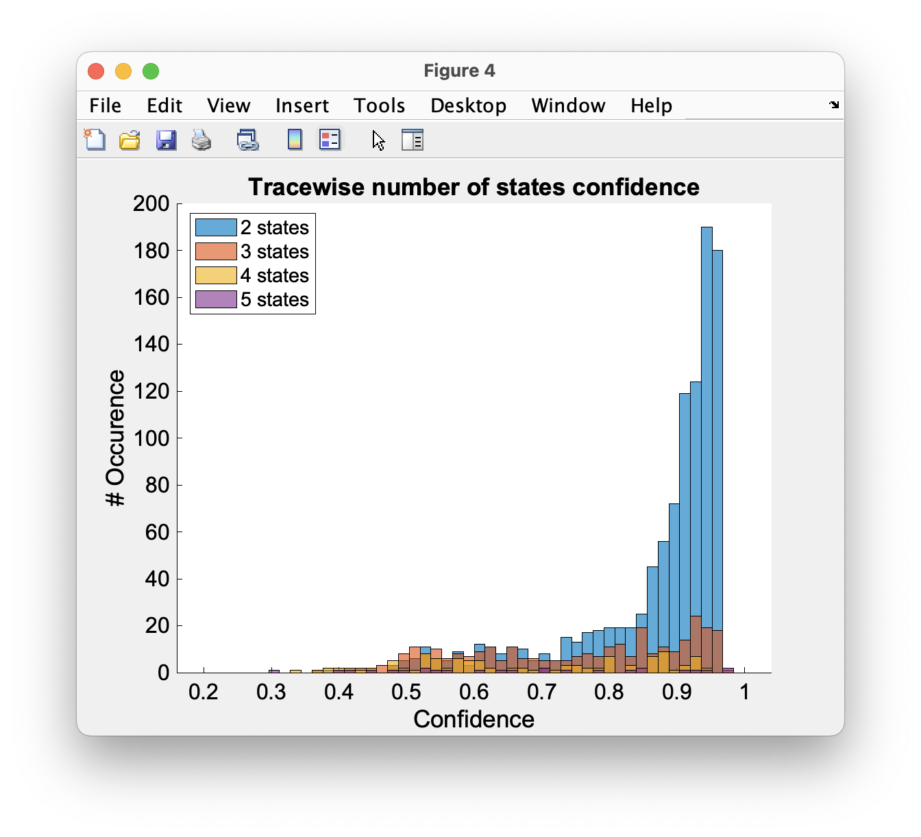
Fig. 32 Number of states confidence for each trace
The predictions of the number of states classifier are used for model selection of the state transition classifier, which subsequently sort all frames in the dynamic traces into state occupancy. Fig. 33 and Fig. 34 show a histogram of trace-wise state confidence and state-wise FRET efficiency respectively.

Fig. 33 State transition confidence
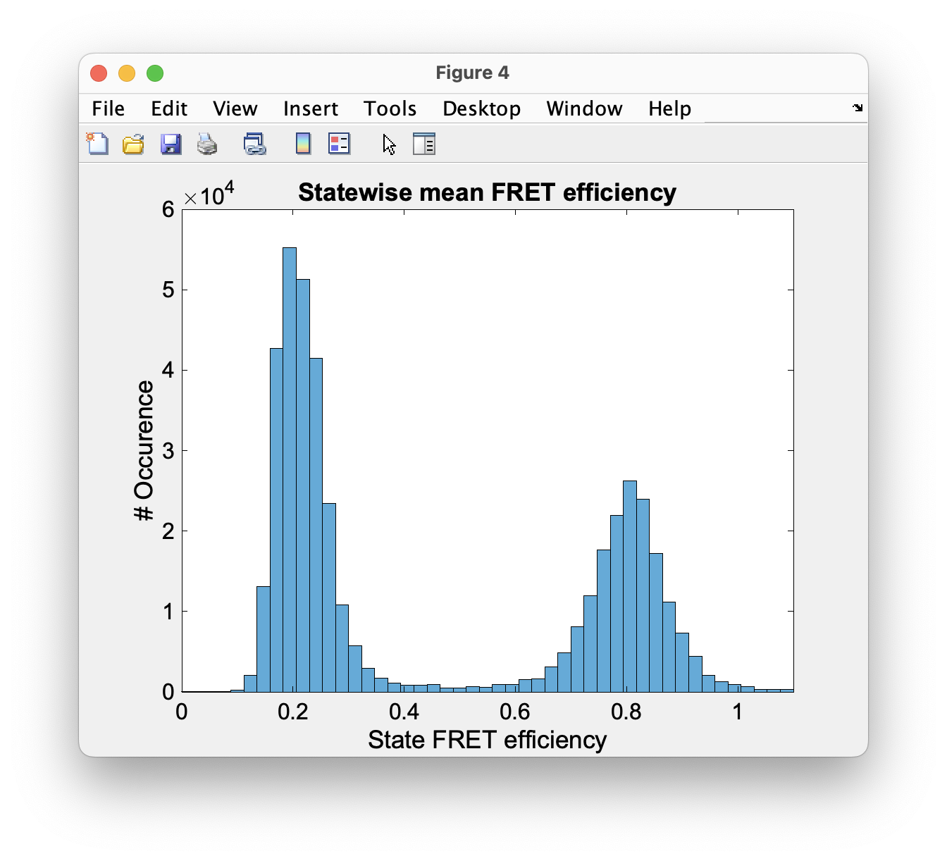
Fig. 34 Statewise mean FRET histogram
After all neural network predictions are completed, the program asks you to choose the number of bins, the confidence threshold and the number of states categories to include in the TDP (Transition Density Plot), as shown on Fig. 35.
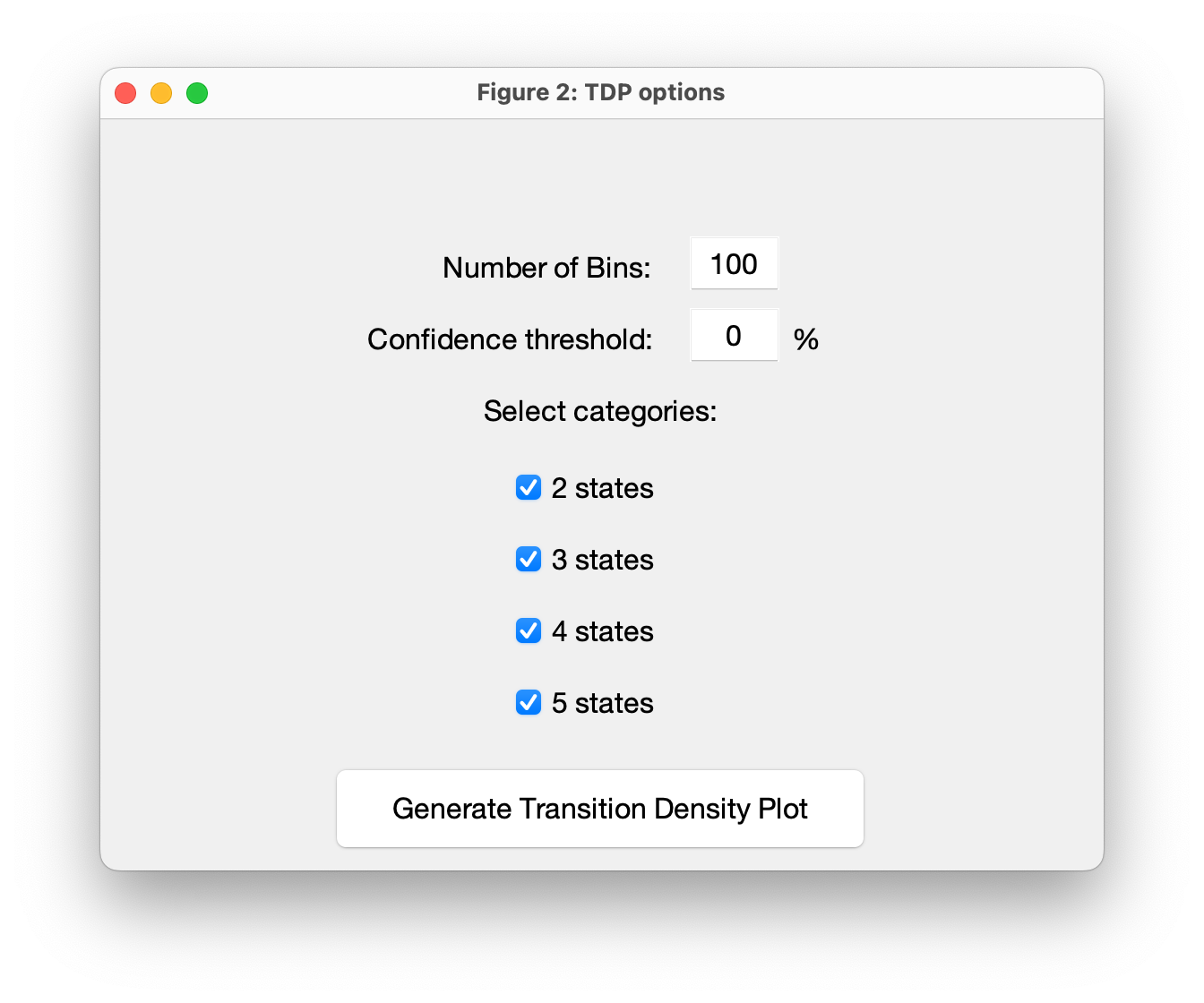
Fig. 35 TDP input parameters

Fig. 36 TDP with live fit panel
When the TDP is generated like the example shown on Fig. 36, by clicking on Select ROI, you can choose a cluster and obtain dynamic information about it. The mean values of dwell time, initial and final FRET, and the number of transitions appear on the next box to the right. The live fit panel below fits the selected dwell times with an exponential function. By choosing the Fit Selection, Fit Upper Triangle or Fit Lower Triangle you can fit the dwell times using the Curve Fitting Toolbox™ from MATLAB (not available in compiled programs!). Plot Dwell times will plot the dwell times of the selected transitions in a histogram. Plot FRET and Plot corr. FRET show you the histogrammed apparent and corrected FRET efficiency of the selection, respectively. In case of 3-color FRET data, the FRET efficiencies of all other dye pairs are shown as well.
Magic button is the fully automated step. You may also intend to take automatic but still separate and different analysis steps without the magic button. That is why a couple buttons are provided on the same table of Deep Learning (Fig. 30). For example, if you would only like to categorize your traces, you can click on the button Categorize Traces. Then with the options provided (Fig. 37) you can select the closest option to your measurement features. You can also leave it as the default option Auto select to have the Deep-LASI recognize the model. Then confirm it by clicking on OK, and after a short while, have all the traces categorized.
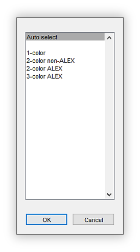
Fig. 37 The options for selecting the closest neural model to the data under analysis
You can also get information about the number of states within traces by clicking on Number of States. Then, the program will ask you to choose whether you want the raw traces or the corrected ones to be evaluated for that. Obviously, prior to choosing the corrected traces option, you should have the traces already corrected. In order to obtain the correction factors or corrected FRET efficiency, one can click on the button Autocorrect. Please note that to do the autocorrection, you should first click on Categorize Traces and then click on Autocorrect. The same is true for the button State Transitions. After categorization, you would first choose the correct model among the options, decide about the process being performed on raw or corrected traces, and have the program informing you about the number of transitions in the category Dynamic (filtered). After having the categories made by the software, you always have the freedom of going through the traces, make any changes, and save the current status of the data set.
Statistics
Selected traces and categories
To get more information about the system under study, Deep-LASI provides statistical information about single molecule measurements. When having traces loaded to the program, by moving on to the Statistics tab (Fig. 38), and selecting any category from the table, one can obtain information about the data quality with several histograms and corresponding fitting results, regarding to fluorophores behavior with brightness, photo-activity time range, and signal to noise ratio. It is especially helpful with knowing about the effects of different parameters in experiments such as the influence of buffer or various background sources.
As you can see on Fig. 39, the left panel of the GUI is divided into four columns, each representing a detection channel. For each channel, five panels are provided to report the number of events for several criteria including: Total signal, Mean BG and Signal, Countrate, Signal to Noise, and Bleaching time.
After having the traces loaded to Deep-LASI, the Selector Table on the right side of the GUI gets updated showing the same sorting table as the user has defined earlier, for an example see the zoomed-in panel on the right side of Fig. 39. Also, the number of columns on the left panel, gets updated depending on the number of channels used for the experiment. For example, for a two-channel measurement, only the first and second columns show histograms, the other two columns will disappear automatically.

Fig. 38 Statistics tab on the main-GUI of DeepLASI

Fig. 39 Statistics environment with subpanels for all channels with the same categories table
You can now choose the desired category to see the histograms for each channel, and obtain the fitting results in the table Fit Results on the bottom right position. The fitting results table will also be divided in separate columns depending on the number of used channels. With clicking on any other category, Deep-LASI will immediately update the whole panels with the fitting results.
An example of created histograms and corresponding fits under the Statistics tab is depicted on Fig. 40. The plots on each column represent the detection channel color, for example Fig. 40 shows the histograms in green, so the reported plots and values are from the data on green channel.
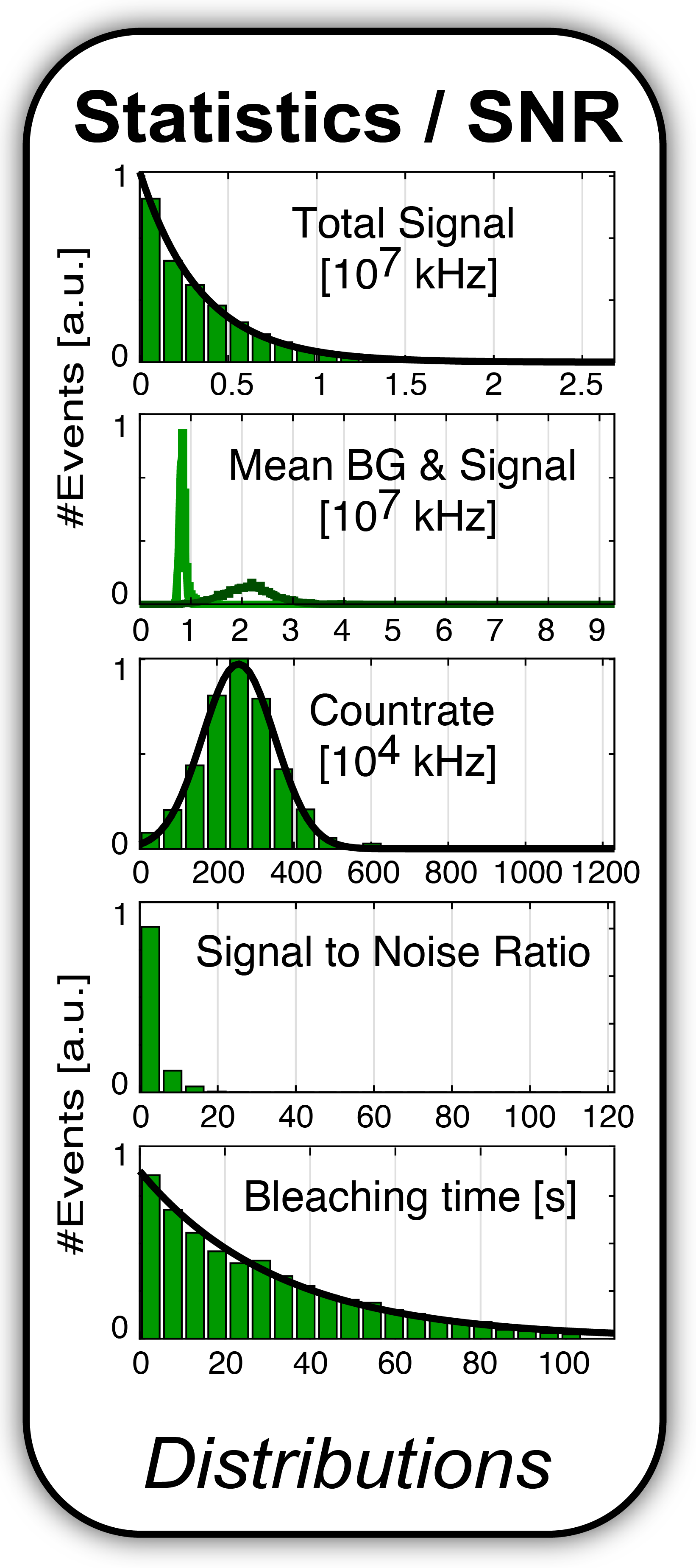
Fig. 40 Histograms showing measurement statistics for green channel
The fit Results table provided on the right side of the statistics GUI, includes measurement criteria listed on Table 7.
Fit Result |
Definition |
|---|---|
File Name |
The data file name given by the user |
\(N_{files}\) |
The number of data files saved in the measurement folder |
Filters |
??? |
\(N_{traces}[Total]\) |
The total number of extracted traces |
\(N_{traces}[filtered]\) |
The number of traces in the selected category |
\(t_{frame}[ms]\) |
The sum of exposure and interframe time |
\(A_{sig}\) |
The number of events of the total signal |
\(A_{1/2}\) |
The total counts on the channel |
\(\mu_{sig}[A.U.]\) |
The mean value of signal |
\(\sigma_{sig}[A.U.]\) |
The standard deviation of signal |
\(\mu_{BG}[A.U.]\) |
The mean value of background |
\(\sigma_{BG}[A.U.]\) |
The standard deviation of background |
\(\mu_{CR}[kHz]\) |
The mean value of count rate |
\(\sigma_{CR}[kHz]\) |
The standard deviation of count rate |
\(\mu_{SNR}\) |
The mean value of signal to noise ratio |
\(\sigma_{SNR}\) |
The standard deviation of signal to noise ratio |
\(A_{bleach}\) |
The number of events of observed bleaching times |
\(t_{bleach,1/2}[s]\) |
The time interval before a flourophore photo-bleaches |
Histograms
Plotting and fitting the results
After having traces categorized with selected regions on each trace, in order to plot various parameters and fitting the distributions, you can move on to the Histograms tab on the main GUI (Fig. 41).

Fig. 41 The Histograms tab on the main-GUI of DeepLASI
As shown on Fig. 42, the provided tab consists of several panels. The panel Plots displays any created graph(s), and in case of fitting them, also fitting results attached to the plot(s). The panel Data Selection shows the same categories created before with the number of traces on each category. On the section Plot Mode, you can choose the desired parameter to be plotted. The provided list of parameters includes apparent and corrected FRET efficiencies, detection efficiency correction factor (gamma), spectral crosstalk and direct excitation correction factors, and stoichiometry in the both apparent and corrected FRET efficiency cases. All the options provided on this whole GUI can be updated or changed any time later while handling and fitting the plots.
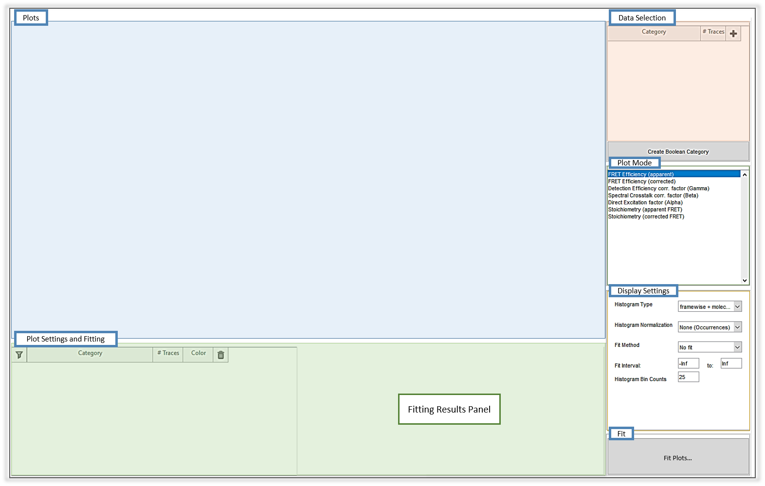
Fig. 42 The Histogram-GUI of Deep-LASI has several sub-windows for plotting data and fitting
On the panel Display Settings one can choose how to show the results considering the various options provided for plotting and fitting (Fig. 43). When creating a plot including the FRET efficiency, you can choose the histogram type from a drop-down menu to be framewise, moleculewise, or both at the same time. A framewise histogram consists of all the FRET efficiencies observed from all the detected molecules on each frame gathered from the whole measured frames, whereas a moleculewise histogram shows the distribution of average FRET efficiencies for each molecule during all the measured frames. Comparing these two types of graphs can give a hint about the presence of conformational changes in the system under study.
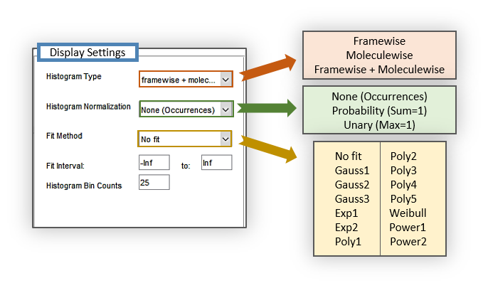
Fig. 43 Various options for plotting and fitting histograms on the panel Display Settings
The second drop-down menu on Fig. 43 includes options about plot normalization. Depending on your purpose of data visualization, you can decide on showing the Y axis without any change, so reporting the number of occurrences without normalization as the default option. You could also normalize the histogram in two different modes. With normalization regarding to probability, the sum of all the possible occurrences is set to one, and we get a probability distribution for the measured values. On the other hand, with the Unary normalization, the highest occurrence will be set to one, and the rest of the values will be shown proportionate to that maximum one.
On the Fit Method drop-down menu, a long list of fitting options is provided to cover a wide range of distribution functions and describe the measured system more precisely. The default is always set to No fit, and the first option is to fit the histogram with a Gaussian function up to three populations. Single and double exponential functions, polynomial function up to five degrees, Weibull distribution, and also first and second power functions are the other fitting options provided (Fig. 43).
When you have the fitting method selected, the next step is to set the Fit Interval, which you can usually use the default range set to infinite numbers unless you have a particular range of values in mind. Finally, you can change the number of bins for plotted histogram(s) depending on the statistics you get.
With all the settings, you can click on Fit Plots and get the fitting results on the allocated panel as you can see on Fig. 42 at the bottom. Sometimes fitting does not happen successfully at first, meaning that the software might fail to fit on the first attempt. In such a case, based on the fitting method and the approximate values visible on the plot, we can guide the fitting results to get closer to the correct values, and then let Deep-LASI do it more exactly. As an example, suppose we had chosen Gauss1 as the fitting method, then a table like Fig. 44 would be produced to report the fitting results. In case the fitting fails, you will get a message as Fit failed, and you can try to fix this issue manually. Meaning that you enter a rough value for a and b with having them fixed by checking on the box beside each of them. This rough values you can get by just checking the maximum value on your y axis, and estimate the corresponding x value for a and b respectively. Now if you click on Fit Plots again, you will get a fitting with the fixed values you entered. Then, one can uncheck the fixing boxes, click on Fit Plots once more, and get the more precise fitting performed by the program. The fitting results will be updated on both the current box and on the plot panel. In case of choosing other fitting methods, the parameters assigned to a, b or c might change, and the user should usually have a slight idea what each parameter would mean in the applied fitting function.

Fig. 44 The fitting results table at the bottom of the histograms tab main-GUI
When you create a plot, the table Plot Settings on the left bottom of the window (Fig. 45) also gets updated. It shows any category that you selected for plotting from which you can choose to be on the plot by checking or unchecking the filtering box on the left side. The third column is to show the number of traces in the present category. The fourth column is to determine the desired color for each plot. By clicking on the colored box, you can set the color as you wish.

Fig. 45 The table for adjusting plot settings
Clicking on the colored box, opens a window like the left one on Fig. 46, letting the user choose a color from the standard ones offered by the program. The recently used colors and a preview of the current choice are also displayed. In case one likes to set a color different from the provided ones, by clicking on the top right corner, the window for custom colors will open with various options. You can use any of the two sliders to choose a desired region of colors. There is also a drop-down menu with four options including: RGB with the scale 0 to 1 which is the default, RGB with the scale 0 to 255, Hex, and HSV. In each selected case, the user has the freedom to set different coloring values or codes.

Fig. 46 The GUI for setting the desired colors for plotting

